武汉加油!中国加油!
2020年第一篇博客,首先来填坑。本项目搭建了Wi-Fi检测信息分析网站,介绍了基于Wi-Fi信号检测的公交OD估计方法。这是本科两个毕设(软件工程+交通工程)的结合。
Origin-destination (OD) data of bus passenger flow is useful for improving the bus service. The OD matrix contains information about where passenger board and alight the bus. It can be used to design a new bus route, new stations, change the route structure, improve vehicle scheduling and driver scheduling (1). Currently, passenger demand information can be obtained through Automatic Passenger Counter (APC) systems (2), Automatic Fare Collection (AFC) systems (3). But those data may only be used to find the origin of passengers and not their destinations, and ride time. According to the Cisco Visual Networking Index: Forecast and Trends, 2017-2022 White Paper predicts that in 2020, more than 53% of IP traffic in the global market will come from Wi-Fi devices. In addition, the report predicts that the number of Wi-Fi access points worldwide will increase year by year, from 64.2 million in 2015 to 432.5 million in 2020 (4). With the popularity of smart mobile communication devices, passengers will carry mobile devices with them during the trip. Mobile devices such as smartphones, tablets, and laptops constantly emit Wi-Fi signals. These signals can be distinguished by the device’s unique Media Access Control (MAC) address. Note that every MAC address is unique to its device. It is possible to obtain an OD matrix by detecting these device’s MAC addresses.
Recently, a large number of studies have been conducted to obtain Bus passenger flow data based on Wi-Fi signals. For collecting Wi-Fi signals data of mobile devices, a Wi-Fi detection system needs to be built, Mikkelsen et al. (5) proposed a rapid prototype of the detection system using a Raspberry Pi and a Wi-Fi network card. As the detected Wi-Fi signals may come from devices outside the bus, classifying them as originating from passenger or non-passenger devices is necessary (5;6;7). Oransirikul et al. (7) proposes a real-time filtering mechanism with received signal strength indication (RSSI) as the filtering parameter, with an accuracy rate of 75%. Some studies use detection data to estimate passenger board and alight stop, and then generate an OD matrix for Wi-Fi devices (3;8). In addition, the algorithms that estimated the actual OD flow matrix based on the Wi-Fi device OD matrix have been proposed (8;9). Ji et al. (8) propose a hierarchical Bayesian model to estimate trip-level OD flow matrices using sampled OD flow data and boarding data provided by fareboxes.
The objective of this paper is to estimate the trip-level OD matrix by detecting Wi-Fi data in the bus combined with passenger boarding and alighting counts. The contributions of this work are as follows:
(1) Design a Maximum Likelihood Estimator (MLE) method to estimate the actual trip-level OD matrices.
(2) Propose an arrival time matching method to infer the OD matrices of Wi-Fi devices.
(3) Developed djtubustool website for Wi-Fi signals data collection, storage, and computation.
The remainder of this paper is organized as follows: Section 2 presents the data collection system, including Wi-Fi sensors, detection data analysis website. Section 3 introduces Methodologies, including detection data filtering methods, Wi-Fi device OD matrices and actual OD matrices estimation methods, and performance metrics. Section 4 introduces the process of empirical evaluation and analyzes its results. Section 5 presents the conclusions and proposes future work.
2.1 System design
The data collection system is divided into two parts, including the hardware system and the data analysis website. The hardware system is responsible for collecting and uploading Wi-Fi data on the bus. After the Wi-Fi sensor completes data collection, this paper develops a data analysis website. This website provides efficient data storage, calculation, and display, as well as passenger boarding and alighting counts of manual surveys. The architecture of the system is shown in Figure 1.

When the detect time reaches a fixed period, the Wi-Fi sensor will switch from the monitor mode to the connect mode and actively establish a connection with the previously set network. Wi-Fi sensors upload data and then switch to monitor mode after the transmission is complete.
The data receiving module on the server side receives the data packet sent by the detection module, and stores it in the database after parsing. Investigators can access the website at any terminal to monitor the Wi-Fi detection data in real-time. After the investigation experiment is completed, the investigators can perform data calculations on the web page, and calculate the OD matrices of the bus route based on the manual survey results and Wi-Fi detection data.
2.2 Hardware system
In the IEEE 802.11 communication protocol, a device needs to be “discovered” by the network before it is connected to a Wi-Fi access point. Probe request management frames are designed to solve the “discovery” problem of access points. When mobile devices are not connected to the access point, mobile devices with Wi-Fi enabled will periodically send probe request frames to actively discover nearby access points. Within the detection range of the Wi-Fi sensor, the Wi-Fi sensor can receive a probe request from a Wi-Fi device in monitor mode and extracts the device’s MAC address. By continuously detecting the probe request frames of the mobile device in the bus, and uploading the collected detection data to the database of the server, real-time detection of the mobile device can be achieved.
The hardware of the data collection system consists of three parts, including Wi-Fi sensors, mobile power bank, and mobile network connections. Figure 2 shows the composition of the hardware of the data collection system.

The Wi-Fi sensor uploads the detected Wi-Fi signal data at a fixed period, and the detection range is about 50 meters. Wi-Fi sensors can collect the following data: source MAC address, destination MAC address and signal strength (RSSI). Source MAC address is the MAC address of the detected device. Destination MAC address is the MAC address of the device to which the packet was sent. Mobile network access points provide network connectivity for data uploads. Power bank provides power for Wi-Fi sensor’s run.
3.1 Data filtering
Since the detected signal data may come from pedestrians, vehicles, and buildings outside the bus, it is necessary to filter the data of the devices outside the bus. Some studies have tried using data pre-processing steps to reduce noise data (5). In this study, from the perspective of the duration of the device detection, it can be considered that the device with a short detection duration may be a device that was briefly detected outside the bus. Therefore, the detection duration is selected as a parameter for filtering signal data. Let T represent the duration of the device detection and represents the minimum duration. MAC address data with device detection duration less than $T_{\min }$ will be removed:
From the perspective of the distance between the device and the sensor, it considers that devices with long distances do not exist in the bus, so the average signal strength is selected as a parameter to filter the signal data. Use to represent the average signal strength of the device, to represent the minimum average signal strength, and the detection device data with the average signal strength less than will be filtered:
3.2 Wi-Fi device OD inference based on time matching
For the inference of the boarding stop of the device, find the stop where the arrival stop time closest to the device’s first detect timestamp, and earlier than the first detect timestamp. For the inference of the alighting stop of the device, find the stop where the arrival stop time closest to the device’s last detect timestamp, and later than the last detect timestamp. The inference process of the boarding and alighting stop of the detection devices is shown in Figure 3.

The OD matrix estimation steps of Wi-Fi devices are as follows:
Step1: Infer the boarding stop of the device. Compare the arrival time of each stop in sequence with the time when the device was first detected, and find the first stop whose arrival time is greater than the first detection time. The previous stop at this stop is considered to be the boarding stop of the device. boarding stop is given by:
Where represents the boarding stop, represents the first detection time, represents the arrival time of the x stop, and k represents the stop number.
Step2: Infer the alighting stop of the device. Compare the arrival time of each stop in sequence with the last time the device was detected, and find the first stop whose arrival time is greater than the last detection time. Consider this stop as the alighting stop for the device. the alighting stop is given by:
Where represents the alighting stop, and represents the last detection time.
Step3: Accumulate the number of devices in Wi-Fi device OD matrix according to the inferred corresponding positions of the boarding and alighting stop:
where represents the number of devices which boarded at and got off at .
Repeat steps 1 to 3 until the data inference for all devices is complete. The Wi-Fi device OD matrix based on time matching can be obtained as shown in Table 1:
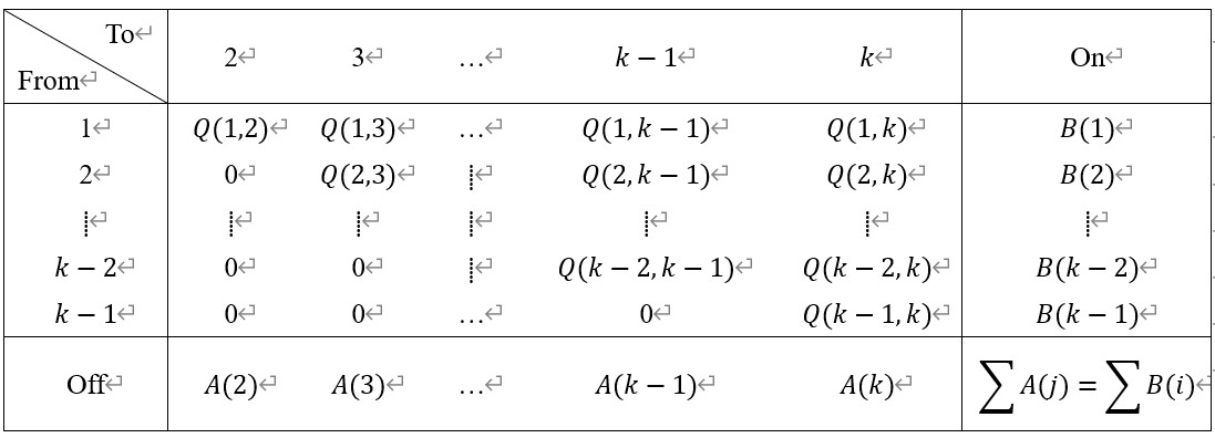
where represents the number of detection devices originating from stop i, and represents the number of detection devices alighting at stop j.
And the bus load L(x) is given by:
where L(x) represents the bus load from stop x to stop x+1, and L(1)=B(1).
3.3 Actual OD estimation
In order to estimate the actual OD matrix using the Wi-Fi detection OD matrix, according to the method proposed by Ben-Akiva (10), a Maximum Likelihood Estimator (MLE) method is proposed in this paper. The following are assumptions for maximum likelihood estimation:
(1) Passengers arrive individually and according to a Poisson process.
(2) There is negligible bias in Wi-Fi OD matrices data.
(3) The boarding and alighting counts are independent of each other.
Assumptions (1) to (3) are considered reasonable in most cases (11). In this study, we usually use a Wi-Fi OD matrix and the boarding and alighting counts for MLE.
As the MLE, the mean value of this Poisson process is the detected arrival rate for OD pair i,j:
Where is the mean value of the Poisson process for passenger arrivals with origin i and destination j, and is the percentage of passenger flows from i to j detected by the Wi-Fi sensor.
The total probability or likelihood of observing all the data is:
Taking the natural log on both sides:
Where C is a constant. Since is also unknown, it is impossible to estimate and at the same time. By assuming that the detect rate is dependent on the origin and destination stop, as the study (10) proposes, we can replace by :
To solve for , we can take derivatives on both sides over , and set the derivatives to zero, and solve the resulting equation:
Therefore, the maximum likelihood estimates for is:
Where is the value of maximum likelihood estimates for each OD pair.
4.1 Experiment design
As shown in Figure 4, this paper selected the Dalian 101 bus route for evaluation. The bus route runs from Malan Square in the west to Dalian Railway Station in the east and has 11 stops. The direction of the route investigated in this study is from Malan Square to Dalian Railway Station.
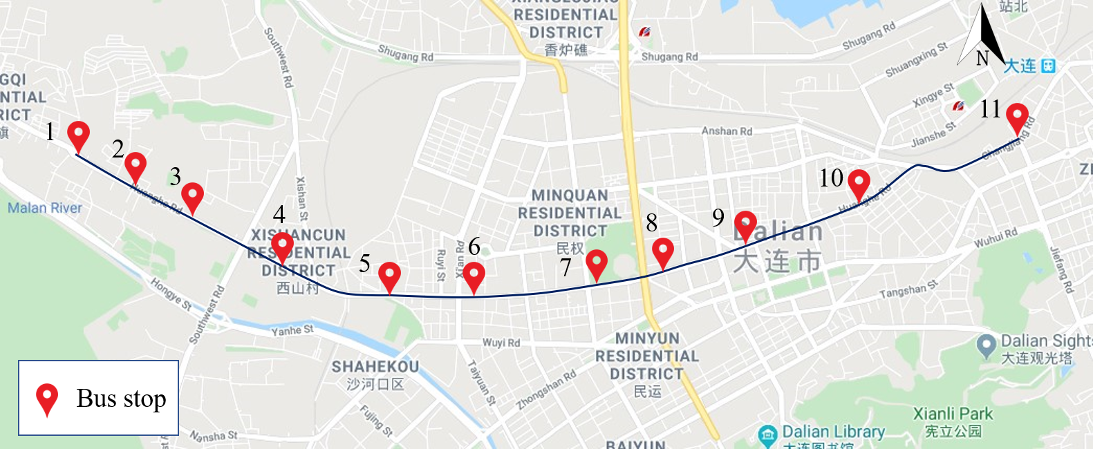
The survey was conducted from April 8 to April 13, 2019, including weekdays and weekends. The survey period includes four periods of 7: 00-8: 00, 8: 00-9: 00, 16: 00-17: 00, and 17: 00-18: 00. The survey data includes Wi-Fi signal data and boarding and alighting counts at each stop. The on-board survey includes the number of passengers boarding and alighting the bus at each stop, the arrival time and the departure time of each stop. A total of 10,517 Wi-Fi signals were detected from 686 mobile devices.
4.2 Data cleaning
The detection range of the Wi-Fi sensor is about 50 meters. When the sensor is installed in the bus, the Wi-Fi signal outside the bus is inevitably detected. In this study, the minimum duration and minimum average signal strength were designed as filtering parameters. The procedure for determining parameter values is as follows:
Step1: Determine a set of parameters according to 10%(40s), 20%(80s), 30%(120s) of the cumulative frequency of the device detection duration and 10%(-94dBm), 20%(-93dBm), 30%(-92dBm) of the cumulative frequency of the average signal strength respectively, and combine them to get 9 filtering parameter pairs as the table 2 shows, use these parameters to filter the data.
Step2: Find the minimum value of the variance of the ratio of the detected Bus load to the actual bus load, and its corresponding filtering parameter value is considered have the most stable filtering effect, which is the optimal filtering parameter value.
Step3: Count the optimal filtering parameter values of each trip dataset, and determine the value of the filtering parameter as the parameter pair that has become the optimal filtering parameter most times.
According to the above steps, 9 sets of candidate parameters are determined to filter the 10 trip datasets, and the number of times that these 9 parameter pairs become the optimal filtering parameters is counted, as present in Table 2.
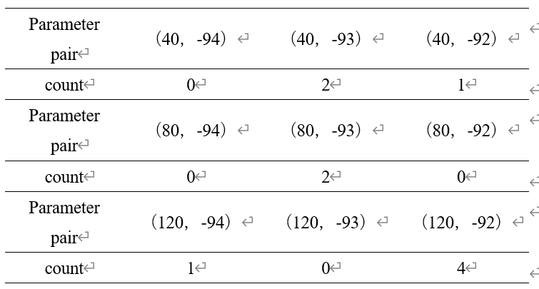
From the statistical results in the table above, the minimum detection duration and minimum average signal strength were determined to be 120 seconds and -92 dBm, respectively.
4.3 Performance metrics
The objective of this paper is to obtain a good OD matrix estimation based on the OD matrix of Wi-Fi devices. Due to the labor-intensive and time-consuming investigation of the actual OD matrix, we cannot directly obtain ground truth OD data for measurement. The bus load is calculated by summing each row and column of the estimated OD, and the accuracy of the estimated OD can be evaluated by comparing the estimated bus load with the actual bus load. The evaluation metrics of bus load uses the average bus load difference G, G is given by:
where represents the estimated bus load between stop n and stop n+1 in trip k, and represents the actual bus loads between stop n and stop n+1. The higher G is, the lower the estimation accuracy is.
4.4 Estimate result
In this part, we compare the performance of the MLE and a proportional fitting (PF) method in terms of bus load of each trip. For comparison, a simple, easy-to-implement proportional fitting (PF) method is also used for evaluation. For each cell of the base matrix multiplied by the proportion of actual to detected boarding counts, the actual OD flow matrix E(i,j) is given by:
where represents the count of passengers boarding at the stop i.
“Structural zero” problem (10) occurred when using the PF method to calculate. The problem is that at a given stop, the number of detected devices boarding the bus is zero, but the number of passengers boarding the bus is not zero, which results in the updated value of OD pairs boarding from this stop still be zero. In this paper, solve this problem by changing the “0” cells of the base matrix to “1”.
Figure 5 shows the estimated and true bus load profiles for each bus trip. Trip1, 3, 5, 7, 9, and 11 are the survey results in the morning (7: 00-8: 00), while trip2, 4, 6, 8, 10, and 12 are the afternoon (16: 00-17: 00) results. For the former, the maximum segments of the bus load are between stop 5 and stop 7, and for the latter, there are two maximum segments that stop 4 to stop 6(for trip 2,6,10) and stop 6 to stop 8(for trip 4,8,12). Obviously, the variation of passenger demand for different periods leads to large trip-level demand variation. In addition, variations in land use near the stop also lead to variations in passenger demand. For example, the sixth stop is Xi’an road stop. It is near a large commercial center with a large number of commuters, so the bus load before the sixth stop in the morning peak is high. Trip 1 to 8 are weekday survey data and trips 9 to 12 are weekend survey data. The survey data has different passengers’ demands on different dates, also leading to the variation of bus load.
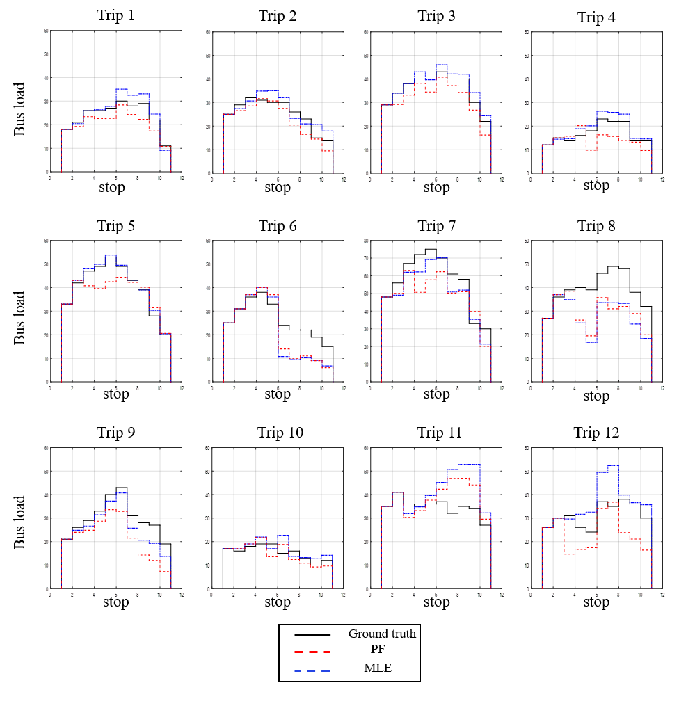
As shown in figure 5, the bus load estimated by the MLE method shows a relatively higher degree of similarity with the corresponding true ones. Therefore, the MLE method can be used to estimate the OD flow with a certain accuracy. As a comparison, the simple PF method may have poor bus load estimates on some bus trips, such as trips 5 and 9.
In order to quantify the estimation error, we statistics the distribution of the estimated bus load error. Figure 6 presents the fitting probability density functions (PDFs) of the estimated error for the MLE and the PF method. Positive error represents the load is overestimated.
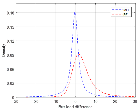
Figure 6 reveals that the MLE method provides better bus load estimates than the PF method. In the figure 6, estimates errors of the MLE method are distributed around “0” mostly, while estimates errors are concentrated around “3” for the PF method. In general, the average absolute error value G is equal to 3.83 for the MLE and 4.96 for the PF. The PF method tends to overestimate the bus load. The PF method has estimation errors that might due to the proportion of passengers boarding at a given stop carrying a Wi-Fi device is not constant.
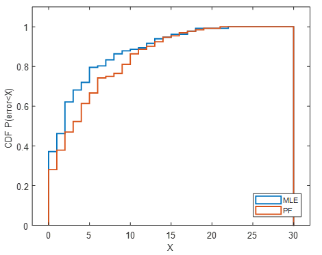
Figure 7 shows the cumulative density functions (CDFs) of the error for the two algorithms base on 12 trips. The figure indicates the MLE method outperforms the PF method. For instance, for about 80% of the bus loads, the MLE method leads to an error lower than 6. For the PF method, the error is lower than 6 only about 67% of the loads. Therefore, MLE can provide a more accurate estimation of the bus load.
5.1 Conclusion
The bus is an important part of the urban public transportation system, and the OD flow data of bus passengers is the basic data for bus operation management and planning. This paper studies the estimation of bus OD matrices based on Wi-Fi signal data. The data collection system built in this paper is divided into two parts, including the hardware system and the data analysis website. The process of collecting, storing, and calculating Wi-Fi data and manual survey data is integrated into the website(www.djtubustool.com), improving the efficiency of conducting survey experiments. And the website is available for anyone who wants to repeat the work in this paper. A method estimating the OD matrices of Wi-Fi devices based on time matching and a Maximum Likelihood Estimator (MLE) method for the actual OD flow matrices estimation are proposed. Data filtering methods based on minimum detection duration threshold and minimum average signal strength threshold are also proposed. According to the empirical evaluation, the MLE method can provide good trip-level OD matrices estimation with the average bus load error is 3.83.
5.2 Future work
Future research needs to determine the uncertainty of the ratio of the detected OD flow to the actual OD flow to improve the accuracy of the estimation. MAC address randomization technology enables a device to transmit multiple MAC addresses. Future research needs to address the identification challenges brought by MAC address randomization.
- Ceder, A. (2016). Public transit planning and operation: Modeling, practice and behavior.
- Ji, Y., Mishalani, R. G., & McCord, M. R. (2015). Transit passenger origin–destination flow estimation: Efficiently combining onboard survey and large automatic passenger count datasets. Transportation Research Part C: Emerging Technologies, 58, 178-192.
- Mishalani, R. G., McCord, M. R., & Reinhold, T. (2016). Use of Mobile Device Wireless Signals to Determine Transit Route-Level Passenger Origin–Destination Flows: Methodology and Empirical Evaluation. Transportation Research Record, 2544(1), 123-130.
- Cisco, V. N. I. (2019). Cisco Visual Networking Index: Forecast and Trends, 2017–2022 White Paper. Porto Salvo, Lisboa. Disponível em:< www. cisco. com/c/pt_pt/about/press/news-archive-2018/20181127. html>, Acesso em, 17.
- Mikkelsen, L., Buchakchiev, R., Madsen, T., & Schwefel, H. P. (2016, September). Public transport occupancy estimation using WLAN probing. In 2016 8th International Workshop on Resilient Networks Design and Modeling (RNDM) (pp. 302-308). IEEE.
- Afshari, H. H., Jalali, S., Ghods, A. H., & Raahemi, B. (2018, November). An Intelligent Traffic Management System Based on the Wi-Fi and Bluetooth Sensing and Data Clustering. In Proceedings of the Future Technologies Conference (pp. 298-312). Springer, Cham.
- Oransirikul, T., Piumarta, I., & Takada, H. (2019). Classifying Passenger and Non-passenger Signals in Public Transportation by Analysing Mobile Device Wi-Fi Activity. Journal of Information Processing, 27, 25-32.
- Ji, Y., Zhao, J., Zhang, Z., & Du, Y. (2017). Estimating bus loads and OD flows using location-stamped farebox and Wi-Fi signal data. Journal of Advanced Transportation, 2017.
- Håkegård, J. E., Myrvoll, T. A., & Skoglund, T. R. (2018, November). Statistical modelling for estimation of OD matrices for public transport using Wi-Fi and APC data. In 2018 21st International Conference on Intelligent Transportation Systems (ITSC) (pp. 1005-1010). IEEE.
- Ben-Akiva, M., Macke, P. P., & Hsu, P. S. (1985). Alternative methods to estimate route-level trip tables and expand on-board surveys. Transportation Research Record, (1037).
- Cui, A. (2006). Bus passenger origin-destination matrix estimation using automated data collection systems (Doctoral dissertation, Massachusetts Institute of Technology).

